Foreword: In this short report, I will make a quick review of L-systems, relying on the book The algorithmic beauty of plants [@TheAB], without talking about the code implementation. The theoretical tools have not changed since the release of the book, it fully covers the state-of-the-art. I will simply explain part of its content. Finally, I have carefully chosen to explain only the parts that are the most interesting to me.

L-Systems

This section presents the simplest class of L-systems, those which are deterministic and context-free, called D0L-systems. One could define L-systems as a formal way of defining developmental processes, that suits well to organic models, and especially plant-development models. More formally, an L-system $G$ is defined as a tuple $\langle V, \omega, P \rangle$, where $V$ is the alphabet of symbols, $\omega \in V^+$ is the axiom, and $P \subset V \times V^*$ is the set of production rules, also called rewriting rules: it takes a character $c \in V$ and returns a string $s \in V^*$. The axiom is the starting character of the L-system, that will fully determine the iteration process. Let $s_i$ be the result of the $i^{th}$ iteration, we define $s_0 = \omega$. An iteration consists of the transformation $s_i \rightarrow s_{i+1}$ defined by the successive transformations of the characters of $s_i$ according to the production set $P$.
For the sake of simplicity, if $x$ and $y$ are two string in $V^*$, then $xy$ is the concatenation of $x$ and $y$.

Example

Let $G_1 = \langle V, \omega, P \rangle$, where $V = {A,B}; \omega = A; P = {A\rightarrow AB, B\rightarrow BA}$. Then the iterations go as follows:

$$\begin{aligned} s_0 &= \omega = A \\\ s_1 &= P(A) = AB \\\ s_2 &= P(A)P(B) \\\ &= ABBA \\\ s_3 &= P(A)P(B)P(B)P(A) \\\ &= ABBABAAB \end{aligned}$$

It almost fully describes an L-system, we now need to interpret the result of an iteration.

Turtle

Turtle graphics, firstly defined by the Logo programming language [@Logo] is a descriptive way of defining computer drawings. We can hence consider an interpretation of some characters (not necessarily all of them) of the alphabet. This will make the turtle move on the screen, and hence draw. For example, $F$ moves forward a step $l$, $+$ turns clockwise the turtle of an angle $\delta$, and $-$ turns counterclockwise the turtle of an angle $\delta$.

Example

If we let $l=1, \delta = 90$, and consider the sentence $$FFF+FF+F+F-F-FF+FFF \ ,$$ then the turtle graphics formalism yields the following, starting in $(0,0)$:

By combining the L-System formalism and the turtle graphics, one can easily generate fractal like patterns, thanks to the recursive structure of L-systems.

A triangle

The above figures shows a fractal-like model where each pattern repeats itself, this comes from the recursive manner of defining an iteration.

More realistic L-systems

This definition of L-systems yields interesting and fractal-like results, but we need to add a branching possibility in order to obtain plant-like results. This is achieved by considering a stack of turtle states and its associated operations: $\texttt{Push}$ and $\texttt{Pop}$. Those two operations are usually represented by the characters $[$ and $]$ respectively. This enhancement yield results shown in fuzzy and aglae.

A fuzzy tree

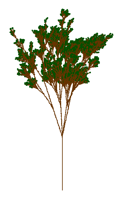
The plant-like pattern appears directly, however, we will explore some enhancement techniques in order to make those more realistic. The issue that one faces with this kind of very simple L-system, is that the plant generated by a L-system is unique, and the artificial regularity is striking. To solve this problem, it is possible to randomize the turtle parameters, the L-system or both.

Randomizing only the turtle parameters has the effect of letting the underlying structure of the results unchanged, while randomizing the L-system itself probabilistically changes the structure, which has the effect of making the result more realistic. Combining the two options is in the end the preferable solution. Such a result is shown in ol_iterations.

An aglae

The list of species being described by L-systems grammar is vastly increasing. Models have been made: cucumber growth [@cucumber], sunflower [@TheAB], barley [@barley], sorghum [@sorghum].

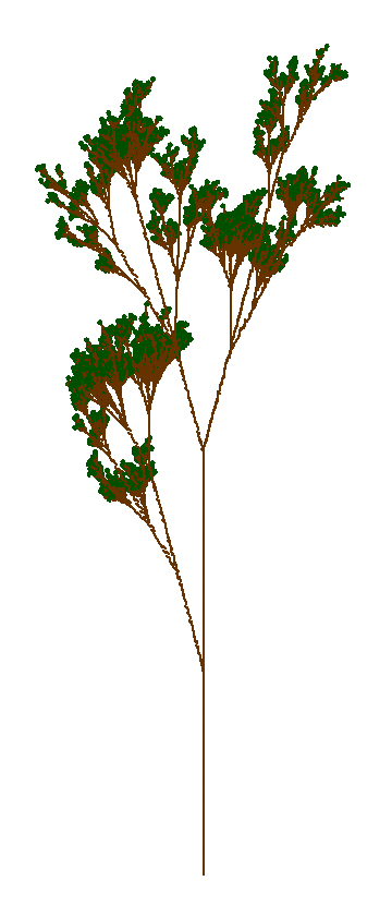
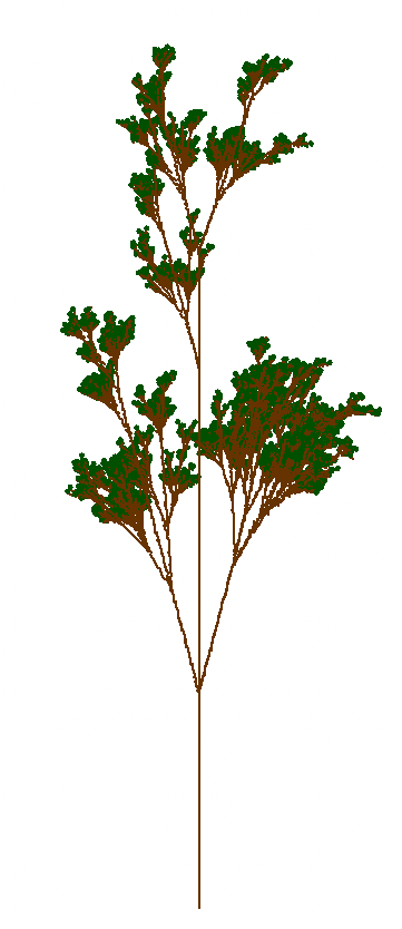
Three iterations of an OL-System (a random tree)

Developmental models of herbaceous plants

In the case of self-similar structures, like trees illustrated in fuzzy, aglae and ol_iterations the synthesis methods based on rewriting rules, are fairly expressive and randomizing strategies fix the problem of unnatural regularity. However, a more general approach is needed to model the large variety of developmental patterns and structures found in nature, especially, it is not possible to obtain the famous sunflower only with 0L-systems. When one observes nature, one sees that the flower development is, although repetitive, highly controlled. For instance, in most of the cases when a flower grows, the stem grows first, and in the end the flower appears. Partial L-systems offer this possibility, especially for the case of single-flower shoot.

Partial L-systems

Partial L-systems can express the vegetative growth of a plant and, after a certain time, the production of the flower. It’s not in essence a new kind of L-systems, in the sense that it is completely defined by a stochastic L-system, but arises from the interpretation of these. Considering the example given in [@TheAB] : $$\label{eq:partial} \begin{aligned} \omega & : a \\\ a \rightarrow & \begin{cases} I [L] a & \text{w.p. } \alpha\\\ I [L] A & \text{w.p. } \beta \end{cases} \\\ A \rightarrow & K \end{aligned}$$

We of course have to have $\alpha + \beta = 1$, $\alpha, \beta \geq 0$. The flower stays in its vegetative phase as long as the rule $a\rightarrow I[L]a$ is applied, and once the rule $a\rightarrow I[L]A$ is selected, the shot stops and the flower appears. It is hence possible to control the average height of the flower, by controlling the ratio $\frac{\alpha}{\beta}$, that can be interpreted as the average height of the result as shown in partial_iteration. Note that the number of iterations is an upper-bound, since the rule $a\rightarrow I[L]A$ is blocking.

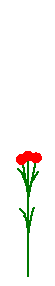
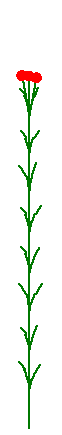
Three iterations of a partial LSystems

Context-sensitive L-systems

Unlike the 0L-systems in which production rules are applied regardless of the context, context-sensitive L-systems, apply rules depending on the context of the character evaluated, that is, its predecessors and successors. This effect is useful in simulating interactions between plant parts. We thus introduce production rules of the form $a_l < a > a_r \rightarrow \chi$, where the rule $a \rightarrow \chi$ is applied if and only if $a$ is preceded by $a_l$ and followed by $a_r$. This allows to move characters (see example), and then introduce a sort of timer in the process. Systems in which we consider only one side for the context are denoted 1L-systems, and the one where we consider the two neighbors of a character, as the following example, are called 2L-systems.

Example (from [@TheAB], shortened):

$$\begin{aligned} \omega & : baaa \\\ b<a & \rightarrow b\\\ a<b> \emptyset & \rightarrow f\\\ b & \rightarrow a \\\ \end{aligned}$$

The first generated sentences are given below:

$$ baaa \Rightarrow % \quad;\quad abaa \Rightarrow % \quad;\quad aaba \Rightarrow % \quad;\quad aaab \Rightarrow % \quad;\quad aaaf \quad $$

Note:

The priority of the rule application not is given by their order of definition, but by the range of their context the broadest context is given priority.

After the $4^{th}$ iteration, the character $f$ appears at the end of the sentence, meaning that if we associate $f$ to the flower and $a$ to the stem, then the flower appears after four iterations at the top of the stem. It is easy, starting from this example, to infer how one can use context-sensitive L-systems to create flower-like models.

Open problems - Miscellaneous

An interesting application of parametric context-sensitive L-systems has been exposed by Hammel and Prusinkiewicz [@diff-eq], is the use of those systems to express numerical solutions to initial value problems for partial differential equation.
Every 0L-system $G$ defines an obvious set of derivations $E(G)$. Those objects, the 0L sequence languages have been studied in [@ROZENBERG1980195].
Open problem: Given two arbitrary OL-systems $G_1$ and $G_2$, is it possible to decide whether $E(G_1) = E(G_2)$?
R. Book conjectured that the answer to the above question is positive.
A locally contenative sequence is a sequence of words in which each word can be constructed as the concatenation of previous words in the sequence.
Open problem: Is it decidable whether an arbitrary DOL-system is locally contenative ?

The above problem constitutes today perhaps the most important open problem concerning DOL systems.

L-systems definitions

Triangle

Parameters: $$\begin{aligned} l & =10 \\\ \delta & = 60 \\\ \end{aligned}$$ System: $$\begin{aligned} \omega & : A \\\ \\\ B & \rightarrow -A+B+A- \\\ A & \rightarrow +B-A-B+ \\\ \end{aligned}$$

Fuzzy tree

Parameters:

$$\begin{aligned} l & =10 \\\ \delta & = 22 \\\ \end{aligned}$$

System: $$\begin{aligned} \omega & : X \\\ \\\ F & \rightarrow FF \\\ X & \rightarrow F-[[X]+X]+F[+FX]-X \\\ \end{aligned}$$

Randomized tree

Parameters: $$\begin{aligned} l & =10 \\\ \delta & = 15 \\\ \end{aligned}$$ System: $$\begin{aligned} \omega & : X \\\ \\\ F & \rightarrow FF \\\ X & \rightarrow \begin{cases} F-[[XC]+XC]+[[XC]+XC]-X & \text{w.p.} \frac{1}{4} \\\ F-[[XC]+XC]+[-FXC]+X & \text{w.p.} \frac{1}{4} \\\ F[+XC][-XC]FX & \text{w.p.} \frac{1}{4} \\\ F[+XC]F[-XC]+X & \text{w.p.} \frac{1}{4} \\\ \end{cases} \end{aligned}$$